Articles
Leakage-Aware Reconstruction of Account-Level Transaction-Amount Distributions via Wasserstein Harmonic Propagation
Abstract
\noindentKeywords: optimal transport; Wasserstein distance; graph-based semi-supervised learning; distribution-valued data; financial transaction data; missing-profile reconstruction.
Introduction
Financial transaction records describe activity intensity, counterparties, payment channels and transferred amounts. Although the underlying data are relational, many analytical tasks operate on account-level summaries. At this level, an account is incompletely characterised by a single total, mean or median: two accounts with the same average transaction amount may allocate their activity very differently across the amount distribution. Representing each account by a probability distribution retains this heterogeneity and is therefore appropriate when the object of interest is a behavioural profile rather than a scalar outcome. More generally, such responses belong to the class of random objects taking values in non-Euclidean metric spaces, for which Fréchet-type methods provide a general statistical framework [1].
This paper studies the reconstruction of partially observed account-level amount distributions. The target profile is observed for some accounts and hidden for others, whereas non-target account attributes remain available for every account. Inference is required for nodes already contained in a fixed graph, making the problem transductive rather than inductive. Three questions motivate the analysis. First, can target-independent account similarities be used to reconstruct a missing distribution? Second, does respecting the geometry of ordered probability distributions improve on global averaging, local-neighbour and Euclidean graph-smoothing benchmarks? Third, how do graph topology, the information used to construct the graph and the proportion of hidden profiles affect reconstruction accuracy?
Graph-based semi-supervised learning provides a natural starting point. Gaussian-field, harmonic-extension and manifold-regularisation methods use smoothness over weighted edges to transfer information from observed to unobserved nodes [2, 3, 4]. Applied coordinatewise, however, conventional propagation treats the entries of a histogram as an ordinary Euclidean vector. This representation ignores the ordering of its support: assigning probability mass to an adjacent amount class should incur a smaller discrepancy than assigning the same mass to a distant class. It may also obscure the distinction between smoothing a vector of proportions and smoothing a probability distribution.
Optimal transport supplies a geometry that incorporates this ordering [5, 6, 7]. In one dimension, the squared 2-Wasserstein distance equals the squared distance between quantile functions, and Wasserstein barycentres admit a quantile-based representation [8]. Distributional graph smoothing can consequently be expressed as harmonic extension in quantile space. [9]developed this principle for semi-supervised propagation of histograms, while [10]applied network-based distributional inference to country-level cyber-risk profiles. The present study transfers this logic to account-level financial behaviour and places particular emphasis on target leakage, benchmark construction and out-of-mask reconstruction accuracy.
The empirical application uses the HI-Small configuration of the synthetic IBM Transactions for Anti-Money Laundering benchmark [11]. Graph representations have proved useful in fraud and AML research because relational dependencies and directed transaction patterns can contain information unavailable from isolated records [12, 13, 14]. The present study nevertheless addresses a different task. The behavioural graph connects accounts according to similarity in account-level covariates rather than using observed transfers as graph edges, and the response is an amount distribution rather than an illicit-activity label. Laundering indicators are never used, and higher amount classes are not interpreted as more suspicious. The synthetic benchmark provides complete and shareable records for controlled methodological evaluation, but it does not establish external validity for operational banking systems.
The study makes four contributions. First, it formulates account-level profile reconstruction as a graph-based learning problem with distribution-valued responses on a common ordered support, evaluating predictions directly with and distances. Second, it imposes a leakage-aware separation between target probabilities and graph-building features, ensuring that a hidden profile cannot affect its own neighbours or incident edge weights. Third, it provides a paired experimental comparison of three graph topologies and four estimators under common masks, separating the effects of graph structure, Wasserstein geometry and multi-step propagation. Fourth, it distinguishes a primary structural-only regime from a sensitivity regime that also contains amount summaries, thereby showing how reconstruction changes when strongly target-aligned side information remains available.
The empirical results qualify, rather than simply confirm, the value of graph propagation. At 20% missingness in the primary structural-only regime, the -harmonic estimator on the Full RBF graph reduces mean error by 30.1% relative to the global benchmark and by 27.3% relative to Euclidean harmonic smoothing. Full RBF and KNN-10 outperform the minimally connected spanning tree, but multi-step propagation provides only a small advantage over a one-step Wasserstein neighbour estimator. When amount summaries are admitted to graph construction, errors fall by 75.7–84.4% relative to the corresponding structural-only graphs and the topology ranking reverses. These results demonstrate both the benefit of distribution-aware geometry and the extent to which apparent predictive performance depends on the information available when the graph is constructed.
The remainder of the paper is organised as follows. Section e̊f{sec:data_profiles} describes the data, preprocessing and account-level profiles. Section e̊f{sec:networks} presents the leakage-aware feature regimes and graph construction. Section e̊f{sec:methodology} develops the Wasserstein harmonic estimator and benchmark methods. Section e̊f{sec:experimental_design} defines the masking and validation protocol, and Section e̊f{sec:results} reports the empirical results. Sections e̊f{sec:discussion}–e̊f{sec:conclusion} discuss the findings, limitations and conclusions. Reproducibility checks and additional diagnostic figures are reported in the appendices.
Data and Account-Level Financial Profiles
Data source and analytical unit
The analysis uses the HI-Small configuration of the IBM Transactions for Anti-Money Laundering benchmark introduced by [11]. The benchmark is generated through an agent-based virtual economy designed to reproduce heterogeneous financial activities, institutional relationships and known laundering typologies. The designation HI refers to a comparatively high proportion of simulated illicit transactions, whereas Small identifies the smallest released scale. All accounts, entities and transactions are synthetic; the data are not anonymised observations of real individuals or institutions.
Although the benchmark was developed primarily for controlled AML model development, the present study does not formulate a laundering-detection problem. Laundering indicators and other benchmark labels are not used in account selection, graph construction or distributional reconstruction. Transaction records are used exclusively to construct account-level amount profiles and the covariates required to define account-similarity networks.
The upstream preprocessing stage starts from 5,078,345 directed transactions recorded between 1 and 18 September 2022. Account identifiers are constructed by combining the bank identifier with the account code. On this basis, the working transaction table contains 984,625 distinct sender-role account keys and 420,640 distinct receiver-role account keys. Because the same account can occur in both roles, these counts are role-specific and must not be added to obtain a total number of distinct accounts.
The account-level analytical file retains senders with at least five outgoing transactions. It contains one row for each of 231,633 sender accounts and summarises 3,892,647 transactions from the working table. Within this file, 100,229 senders have at least 20 outgoing transactions; this subset defines the eligible population for the reconstruction experiment. The distinction between the transaction-level source table, the account-level analytical file and the experimental sample is reported explicitly in Table e̊f{tab:data_preprocessing}.
The sender account is the statistical unit of analysis. For sender , let
index its outgoing transactions during the observation window, and let denote the amount associated with outgoing transaction . Incoming transactions are not combined with outgoing transactions when constructing the target profile. The analysis therefore characterises how an account distributes its outgoing activity across ordered amount classes; it does not estimate account balances, net flows or overall financial positions.
Receiver identifiers and payment formats are retained only to construct the account-level covariates described in Section e̊f{sec:networks}. Transaction timestamps delimit the common observation window, but the experiment treats each account as a static aggregate and does not model the temporal ordering of payments within that window. Identity-related attributes and synthetic laundering labels do not enter the analysis.
| Quantity | Value |
|---|---|
| Working transaction table | |
| Transactions after preprocessing | 5,078,345 |
| Distinct sender-role account keys | 984,625 |
| Distinct receiver-role account keys | 420,640 |
| Observation window | 1–18 September 2022 |
| \addlinespace Account-level analytical file | |
| Senders with | 231,633 |
| Transactions represented for senders with | 3,892,647 |
| Senders with | 100,229 |
| \addlinespace Experimental sample | |
| Accounts selected for the experiment | 1,000 |
| Activity strata used in sampling | 10 |
| Accounts sampled per stratum | 100 |
| Ordered amount classes | 4 |
| Mean transaction count | 23.84 |
| Standard deviation | 6.25 |
| Median transaction count | 21 |
| Interquartile range | 20–28 |
| Observed range | 20–63 |
Ordered amount classes and empirical profiles
Let denote the multiset of positive outgoing transaction amounts in the working table, and let be its empirical distribution function. For , define the global empirical quantile as
The positive amount range is partitioned into four common classes using the three empirical quartiles:
The right-closed convention assigns every observation lying on a cut-point to a unique class. Repeated values at a quartile boundary can therefore make the realised class frequencies differ slightly from 25%, but cannot create ambiguous assignments.
The three internal cut-points are 184.48, 1,414.54 and 12,297.84 in the native numerical scale of the amount field. The benchmark contains transactions in multiple currencies, while the supplied preprocessing pipeline applies no exchange-rate conversion. These cut-points are consequently used to define reproducible global ranks within the processed dataset, not universally comparable monetary thresholds. Combining unconverted currency amounts is a limitation of the present representation and precludes an economic interpretation of the numerical boundaries themselves.
The four classes are therefore denoted Q1–Q4 rather than being assigned labels such as “low risk” or “critical risk.” They encode relative position in the pooled amount distribution and carry no intrinsic AML, credit-risk or regulatory interpretation.
The empirical amount profile of sender account is the four-dimensional probability vector
where is the indicator function. By construction, and , so . Equivalently, the account can be represented by the empirical probability measure
where is a unit point mass at class .
All accounts are evaluated using the same global cut-points, which makes their profiles directly comparable. The cut-points are fixed before the missing-profile experiments and remain unchanged across all replications and masking rates. Masking an account therefore changes only whether its profile is available to the reconstruction procedure; it does not change the definition of the reconstruction target.
The ordered support and its ground metric are
This metric assigns unit cost to movement between adjacent classes and a larger cost to movement across more distant classes. The coding expresses ordinal separation only and does not assume equal monetary spacing between adjacent classes. This distinction underlies the Wasserstein formulation developed in Section e̊f{sec:methodology}.
Activity-stratified experimental sample
Constructing a dense affinity matrix for all 100,229 eligible senders would require evaluating more than five billion distinct account pairs. Because the objective is a controlled reconstruction experiment rather than population-wide estimation, the analysis uses a fixed sample of 1,000 accounts. The eligibility threshold limits the discreteness and sampling variability of the empirical profiles while preserving a large population from which to sample.
To retain coverage across the observed activity distribution, eligible senders are ranked by and divided into ten equal-frequency activity strata. Ties are resolved deterministically according to their order in the account-level file. Exactly 100 accounts are sampled without replacement from each stratum using pseudorandom seed 123. Because the strata contain nearly equal numbers of eligible accounts and use equal quotas, inclusion probabilities are approximately constant while representation across the activity range is guaranteed. The stratum identifier is used solely for sample construction and is not included among the graph features or target variables.
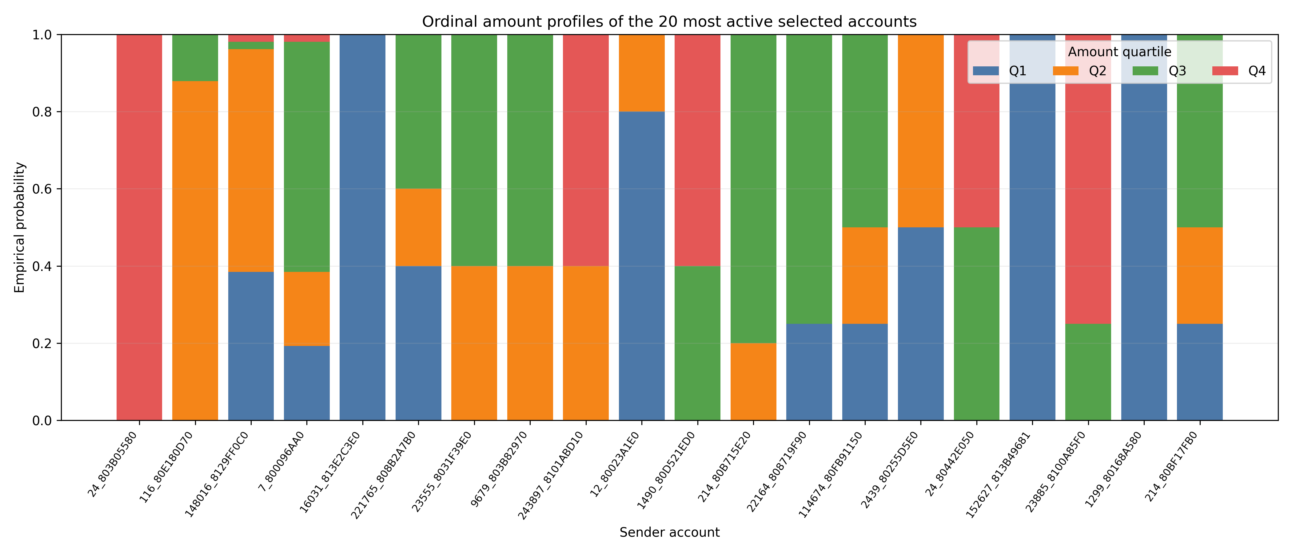
The selected accounts have a mean of 23.84 outgoing transactions ( ), a median of 21, an interquartile range of 20–28 and an observed range of 20–63. Their mean empirical class probabilities are 0.262, 0.279, 0.231 and 0.228 for Q1–Q4, respectively. These account-weighted means need not equal the transaction-level quartile shares, because each account receives equal weight irrespective of its transaction count.
Of the 1,000 selected accounts, 51.6% place all observed outgoing transactions in a single amount class. These profiles lie at vertices of the simplex ; the remaining accounts assign positive mass to two or more classes. The concentrated profiles are retained rather than smoothed during preprocessing. They constitute a demanding part of the reconstruction problem, because assigning mass to a distant ordinal class incurs a larger transport cost than an error confined to adjacent classes.
Figure e̊f{fig:account_profiles} displays the 20 accounts with the highest outgoing transaction counts within the fixed experimental sample. The figure is descriptive: the displayed accounts are chosen only after the 1,000-account sample has been fixed and receive no special treatment during estimation.
\FloatBarrier
Banking Behavioural Network Construction
The graphs considered in this study are behavioural similarity graphs rather than transaction-flow networks. Each node represents one sender account, and an edge indicates similarity between two accounts with respect to a specified set of account-level covariates. An edge does not imply that the corresponding accounts exchanged funds directly. The graphs instead encode proximity in behavioural feature space, which is subsequently used to propagate partially observed distributional profiles.
Leakage-aware feature regimes
Let denote the covariate vector used to position account in behavioural feature space, and let denote its target amount-distribution profile. None of the four target probabilities is included in . The exclusion applies not only to the final distance calculation but also to imputation, standardisation, neighbourhood selection and affinity construction.
This separation is essential to the masking experiment. If the graph were constructed using , or any direct transformation of its four coordinates, a nominally hidden account would continue to influence its own neighbourhood and incident edge weights through the unavailable response. Reconstruction accuracy would then partly reflect information already encoded in the graph rather than propagation from genuinely observed accounts.
Graph construction is performed once for each feature regime before the repeated masking experiments. The resulting feature matrix, pairwise distances and graph weights remain fixed across missingness levels and replications. Only the availability of the target profiles changes between replications. The experiment is therefore transductive: the non-response covariates are assumed to remain available for every account, including accounts whose amount profiles are masked.
The primary specification, denoted \textsc{Core Structural}, uses three account-level covariates: e̱gin{enumerate} \item the number of outgoing transactions; \item the number of distinct receivers; and \item the number of distinct payment formats. \end{enumerate} These features describe activity intensity and interaction diversity without directly summarising how transaction amounts are distributed across Q1–Q4. They may be statistically associated with the target profile, as useful predictors should be, but they do not reveal the allocation of probability mass across the four target classes. Results obtained under this regime are therefore treated as the primary evidence.
A second specification, denoted \textsc{Extended Amount Sensitivity}, augments the structural covariates with total, mean, median and standard deviation of outgoing transaction amounts. These variables are calculated from the same underlying amounts used to form the target profile and can consequently act as strong proxies for its location and dispersion. Their inclusion is compatible with the masking protocol only under the operational assumption that these summaries remain observable when the histogram itself is unavailable. This is a substantially richer information setting. Results from this regime are therefore reported as a sensitivity analysis and are not used as the principal assessment of reconstruction performance.
For feature , the non-negative raw value is first transformed as
The logarithmic transformation limits the influence of highly active accounts and reduces the right skew characteristic of count and amount variables. Any missing transformed value is replaced by the median of the observed values of the same feature. The resulting columns are then standardised:
where denotes the median-imputed value and and are the empirical mean and scale estimated from the 1,000 sampled accounts. These transformations use the covariates of all sampled nodes, consistent with the transductive design. Because no target-profile coordinate enters the operation, preprocessing does not reveal the masked response.
Let denote the resulting standardised feature vector. Pairwise dissimilarity is measured using Euclidean distance,
The distance matrix is converted into a symmetric, locally scaled affinity matrix following [15]:
with . Here, is the distance from account to its tenth nearest distinct neighbour. Unlike an RBF kernel with one global bandwidth, local scaling allows accounts located in dense and sparse regions of feature space to use different effective neighbourhood radii. This reduces sensitivity to heterogeneous feature-space density and to the different concentration patterns of the two feature regimes.
The implementation includes two numerical safeguards. If the tenth-neighbour distance of an account is zero or non-finite, it is replaced by the median of the positive finite local scales. In addition, the exponent is capped at 50 before exponentiation, giving a smallest positive numerical affinity of . These safeguards prevent division by zero and numerical underflow without changing the ordering of ordinary pairwise affinities.
Graph topologies
Let be the common set of sampled accounts and let be the locally scaled affinity matrix. Three undirected weighted graphs are constructed from the same within each feature regime. The node set, feature preprocessing and affinity definition are therefore held constant; only the rule used to retain edges changes.
e̱gin{enumerate} \item Full RBF. Every unordered pair of distinct accounts is connected. The graph therefore contains edges and retains the complete affinity structure. It represents a dense global-smoothing regime in which even behaviourally distant accounts remain connected, although potentially with very small weights.
\item KNN-10. Let denote the ten nearest neighbours of account according to . An undirected edge is retained when either account selects the other:
This union symmetrisation preserves all directed nearest-neighbour relations and generally produces more than but no more than undirected edges. Retained edges keep their original locally scaled RBF weights.
\item MST. A minimum spanning tree is computed from the complete Euclidean distance matrix using Kruskal's algorithm. Its retained edges are subsequently assigned the corresponding RBF affinities . The MST is connected by construction and provides the sparsest possible connected comparison. When two distinct accounts have identical standardised feature vectors, their zero distance is replaced, for tree ordering only, by times the smallest positive pairwise distance. The retained edge still receives its original RBF affinity. \end{enumerate}
Distance ties are resolved deterministically to prevent graph construction from depending on library-specific ordering. For KNN-10, candidate neighbours are ordered first by distance and then by their fixed node index. For MST, candidate edges are ordered lexicographically by before the Kruskal scan. Node indices are fixed after the seeded account sample has been formed. Consequently, the same selected sample and configuration produce the same retained-edge sets when distances are tied.
These constructions represent three distinct smoothing geometries: dense global connectivity, sparse local neighbourhoods and minimal connectivity. Graph construction is known to affect the spectrum, connectivity and regularisation behaviour of graph-based and semi-supervised estimators [4, 16]. The three topologies were specified before examining reconstruction performance; none was selected post hoc as a universally preferred graph.
For an undirected graph , the unweighted degree of node is
whereas its weighted degree, or strength, is
Table e̊f{tab:network_metrics} reports the number of retained edges, edge density, connected components, largest-component size, mean unweighted degree and mean weighted degree for each feature-regime and topology combination.
| Feature regime | Graph | Edges | Density (\ Components | Largest component | Mean degree | Mean weighted degree | |
|---|---|---|---|---|---|---|---|
| \multirow{3}{*}{Core Structural} | Full RBF | 499,500 | 100.000 | 1 | 1,000 | 999.000 | 282.346 |
| KNN-10 | 9,268 | 1.855 | 5 | 470 | 18.536 | 17.986 | |
| MST | 999 | 0.200 | 1 | 1,000 | 1.998 | 1.962 | |
| \multirow{3}{*}{Extended Amount Sensitivity} | Full RBF | 499,500 | 100.000 | 1 | 1,000 | 999.000 | 8.503 |
| KNN-10 | 6,384 | 1.278 | 1 | 1,000 | 12.768 | 6.292 | |
| MST | 999 | 0.200 | 1 | 1,000 | 1.998 | 1.622 |
The two feature regimes produce markedly different affinity structures even when the topological construction rule is unchanged. In particular, both Full RBF graphs contain every possible edge, but their mean weighted degrees differ substantially because the additional amount summaries alter pairwise distances and local scales. Edge count alone therefore does not characterise the effective strength of graph smoothing.
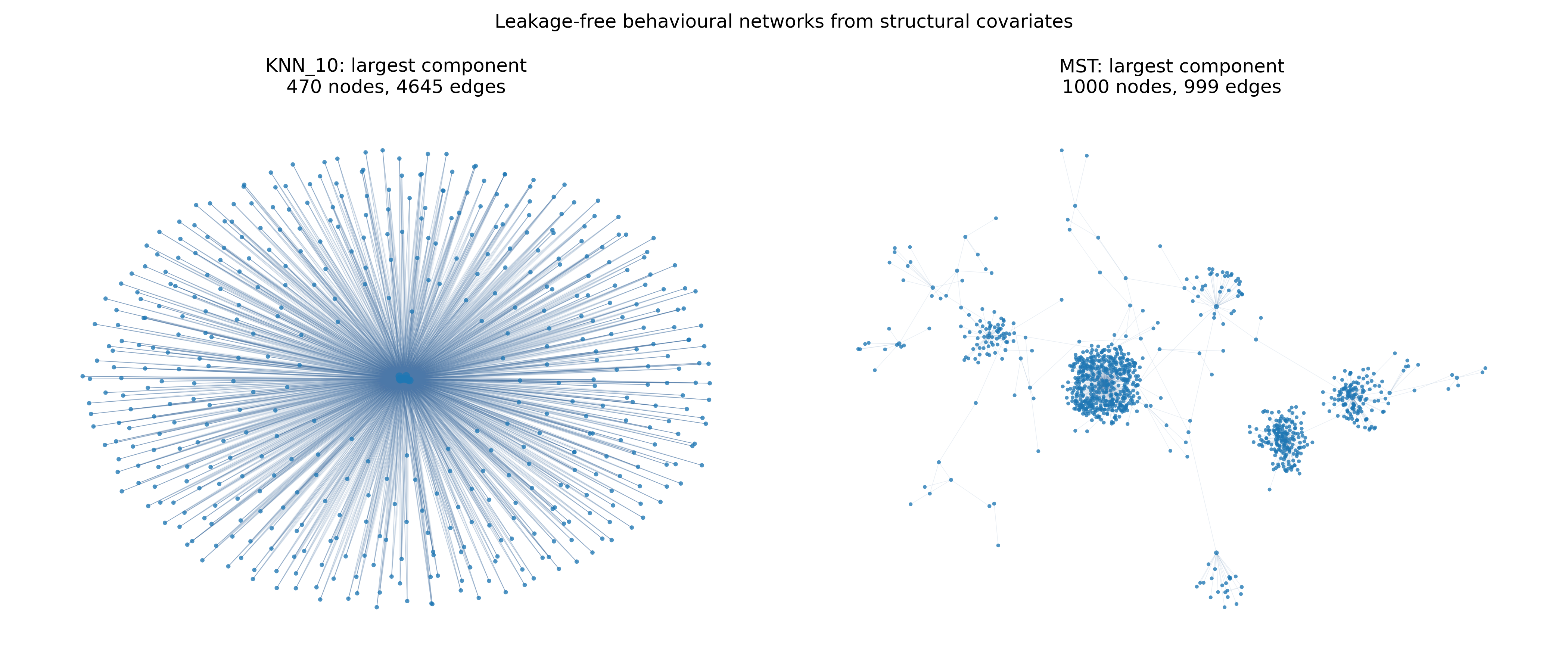
The \textsc{Core Structural} KNN-10 graph contains five connected components, the largest of which contains 470 accounts. All other graphs are connected. A graph-harmonic reconstruction requires each component containing hidden accounts to retain at least one observed profile. This condition was satisfied in every realised masking replication: no component-level fallback was activated. Had an entirely unobserved component occurred, its hidden nodes would have received the global mean of the observed values in the relevant representation, as specified in the reconstruction algorithm.
Figure e̊f{fig:network_structures} shows the largest connected component of the KNN-10 graph and the complete MST under the \textsc{Core Structural} regime. The Full RBF graph is omitted because displaying all 499,500 edges would be visually uninformative. Node positions are generated solely for visualisation using an unweighted force-directed layout; they are not used to calculate distances, affinities or predictions. Node sizes are scaled by the square root of unweighted degree.
\FloatBarrier
Wasserstein Propagation for Distributional Reconstruction
The reconstruction target associated with each account is a probability distribution rather than a scalar or an unordered class label. Treating the four probability masses independently would ignore the ordering of the amount classes and would assign the same discrepancy to errors between adjacent and distant classes. The proposed method instead uses the Wasserstein geometry of probability measures, which incorporates the ground distance between Q1–Q4 directly into estimation.
One-dimensional Wasserstein geometry
For account , let
be the empirical distribution defined on the ordered support with ground metric . Its cumulative distribution function is
and its generalised inverse, or quantile function, is
For probability measures on the real line and , the -Wasserstein distance admits the exact quantile representation
This identity avoids explicit estimation of a transport plan and is particularly convenient for ordered univariate distributions [5, 6, 7].
The estimator is based on squared distance. In one dimension, if are assigned non-negative weights satisfying , their barycentre has quantile function
Thus, averaging quantile functions produces the distribution that minimises the weighted sum of squared distances [8]. This property is the key reason for using during graph propagation: local Wasserstein barycentres reduce to ordinary weighted averages in quantile coordinates.
The integrals in Equation are evaluated numerically on the fixed midpoint grid
Each empirical distribution is represented by the row vector
For an observed account, every coordinate of belongs to because the original distribution is supported on the four ordinal classes. The discrete approximations to and are
These are midpoint approximations to the corresponding integrals and are used consistently for model fitting and evaluation.
Weighted averages of observed quantile functions may take values between the original support points. Such intermediate values are admissible: a non-decreasing function with values in remains the quantile function of a valid probability distribution on the continuous interval joining the ordinal support points. Retaining these values during estimation avoids premature projection onto the four original classes and preserves the displacement structure of Wasserstein barycentres.
The primary evaluation metric is because its square corresponds to the discrepancy minimised by the proposed graph energy. The complementary metric penalises ordinal displacement linearly rather than quadratically and is therefore less sensitive to a small number of large class displacements. Reporting both metrics provides a robustness view of reconstruction error under two transport costs.
Graph-harmonic Wasserstein extension
Let be the common node set of a behavioural similarity graph, and partition it as
where is the set of accounts whose target distributions remain observed and is the set whose profiles are masked. Let denote one of the symmetric non-negative adjacency matrices constructed in Section e̊f{sec:networks}.
Write for the matrix whose th row is . The proposed estimator minimises the discrete graph energy
subject to the boundary conditions
The factor corrects for double counting in the symmetric adjacency matrix, while places each pairwise contribution on the scale of the discretised squared Wasserstein distance. Neither constant changes the minimiser.
By Equation , the energy can equivalently be written as
The estimator therefore seeks a distribution-valued assignment that is smooth with respect to the behavioural graph while reproducing the observed distributions exactly. It is a one-dimensional quantile implementation of graph-based Wasserstein propagation [9].
For a hidden node , differentiation of Equation gives
If is the weighted degree of node , then
Each hidden quantile vector is therefore the locally weighted barycentre of its graph neighbours. Unlike a one-step neighbour estimator, the neighbours in Equation may themselves be hidden, allowing information to propagate along multi-edge paths.
Let
be the weighted-degree matrix and row-normalised transition matrix, respectively. After partitioning and according to and , the harmonic equations become
Provided that every connected component containing hidden nodes also contains at least one observed node, the unregularised system has the unique solution
This is the distribution-valued analogue of classical Gaussian-field and harmonic-function label propagation [2, 3].
The numerical implementation solves
where the small ridge term is introduced solely to stabilise the sparse linear solve. The value is sufficiently small that it is not treated as a substantive smoothing parameter. The system is solved separately within each connected component, avoiding artificial propagation between disconnected regions of the graph.
If a component contained hidden nodes but no observed anchor, the harmonic boundary-value problem would be unidentified within that component. The implementation assigns the mean observed quantile function
to its hidden nodes and records the number of components for which this rule is required. The same deterministic fallback is used if a sparse solve fails or returns a non-finite value. No component-level or numerical fallback was activated in any reported replication.
For the unregularised system, the solution is a weighted combination of non-decreasing observed quantile functions and therefore remains non-decreasing. The numerical ridge and finite-precision solution can produce negligible violations of the theoretical range or monotonicity constraints. Predicted coordinates are therefore clipped to and monotonised using
All reported reconstruction errors are calculated directly from the resulting quantile vectors using Equations and . Conversion back to four-class probabilities is used only for graphical presentation. Specifically, predicted quantile coordinates are assigned to Q1–Q4 using the midpoint boundaries , and , and the proportion assigned to each class defines the displayed probability:
where
This projection is not used during graph propagation and does not affect the reported or errors.
Comparator estimators
Four estimators are evaluated under exactly the same account masks, feature regimes and graph constructions. The comparators are chosen to separate the contribution of graph information, multi-hop propagation and Wasserstein geometry.
e̱gin{enumerate} \item Global Probability. The observed probability vectors are averaged in the original simplex:
Every hidden account receives , which is then converted to a 128-point quantile vector for evaluation. This graph-independent comparator measures performance when account heterogeneity is ignored.
\item \textbf{Local One-Step.} Each hidden account receives the weighted barycentre of its immediately observed neighbours:
If is empty or its total weight is zero, the method uses the mean observed quantile function . This comparator uses Wasserstein geometry but does not transmit information through hidden intermediate nodes.
\item Euclidean Harmonic. Let denote the matrix whose th row is . Classical harmonic extension is applied coordinatewise to the four probability masses:
Predicted coordinates are clipped at zero and renormalised to sum to one. A non-finite or zero-sum row receives the global probability vector . The resulting probability vectors are converted to quantile vectors before evaluation. This method uses the same graph, ridge and multi-hop harmonic smoothing as the proposed estimator but treats Q1–Q4 as four Euclidean coordinates rather than as ordered locations.
\item \textbf{ Harmonic.} The proposed estimator applies Equation directly to the 128 quantile coordinates. It combines multi-hop graph propagation with the ordinal transport geometry of the target distributions. \end{enumerate}
The comparison has a factorial interpretation. Global Probability provides a graph-free reference; Local One-Step introduces graph-local distributional information without multi-hop propagation; Euclidean Harmonic introduces multi-hop propagation without Wasserstein geometry; and Harmonic combines both elements. Differences between the two harmonic methods therefore isolate the effect of representing the target in Wasserstein rather than Euclidean probability coordinates, while differences between Local One-Step and Harmonic assess the contribution of propagation beyond directly observed neighbours.
Experimental Design
The experimental design evaluates the ability of each method to reconstruct complete account-level amount distributions when the target profile is unavailable for a subset of accounts. The selected accounts, behavioural covariates and graph structures are held fixed throughout the experiment. Randomness enters only through the repeated selection of accounts whose target profiles are masked.
Repeated account-level masking
Let denote the fixed set of sampled accounts. Three missingness rates are considered:
For missingness rate and replication , with , a hidden set
is sampled uniformly without replacement, with size
Because , the three conditions hide exactly 100, 200 and 300 account profiles, respectively. The complementary set
contains the accounts whose distributions remain available to the reconstruction method.
Sampling without replacement applies within each replication: an account cannot be selected twice in the same hidden set. Across replications, however, the masks are redrawn and an account may therefore be hidden in more than one replication. Masks for the three missingness rates are generated as separate draws and are not constrained to be nested. Thus, the 20% hidden set is not necessarily a superset of the corresponding 10% hidden set.
A dedicated pseudorandom number generator is initialised with seed 123 for the masking stage. Given the fixed ordering of the selected accounts, the seed fixes the complete sequence of masks. Mask selection does not depend on account covariates, graph position or the target distribution. The experiment therefore implements account-level missingness completely at random within the fixed 1,000-account sample.
When an account is included in , its entire probability vector and corresponding quantile representation are withheld from the estimator. Its non-response covariates remain available, consistently with the transductive setting described in Section e̊f{subsec:feature_regimes}. Graphs and edge weights are not recomputed after masking.
For a given pair , exactly the same hidden and observed account sets are used for: e̱gin{itemize} \item both feature regimes; \item all three graph topologies; and \item all four reconstruction methods. \end{itemize} This common-mask design creates paired comparisons. Differences between two methods or graphs within replication are evaluated on exactly the same hidden accounts and are therefore not confounded by variation in mask difficulty. Pairing also reduces Monte Carlo variability in estimated performance contrasts.
Account- and replication-level errors
Performance is evaluated exclusively on the hidden accounts. For hidden account , let
be the true quantile vector and let
be its reconstruction. The account-level discretised Wasserstein errors are
These errors are calculated after applying the range and monotonicity corrections described in Section e̊f{subsec:wasserstein_harmonic}. No projection to four-class probabilities is performed before evaluation.
For metric , the account-level errors are first averaged within each replication:
This produces one performance value for each combination of feature regime, graph, method, missingness rate and replication. The principal summaries are then calculated across the replication-level means:
Let
denote the sample variance of the replication-level means. The reported two-sided 95% interval is
where is the corresponding Student- critical value.
This hierarchical aggregation prevents the much larger number of hidden account errors from being treated as if they were independent experimental replications. The replication mean, rather than the individual account, is the Monte Carlo unit used for uncertainty summaries.
The intervals in Equation quantify variation across the repeated random masks, conditional on the selected accounts, feature matrices and graph structures. They do not incorporate uncertainty arising from the initial account sample, from generation of the synthetic transaction dataset, or from alternative preprocessing and graph hyperparameters. They are therefore interpreted as conditional Monte Carlo intervals for masking variability rather than as population-level confidence intervals.
Paired statistical comparisons
Paired comparisons are computed for and at each of the three missingness rates. The primary inferential comparisons reported in the main text are restricted to the central condition, , and to replication-level mean error. The corresponding tests are retained as secondary robustness results. Restricting the main comparisons to one missingness rate avoids presenting the three masking levels as independent experimental samples and provides a common reference condition with 200 hidden accounts per replication.
For two configurations and , the paired difference in replication at missingness rate is defined as
Under this convention, a negative value favours configuration , whereas a positive value favours configuration .
The null hypothesis of no systematic paired difference is assessed using a two-sided Wilcoxon signed-rank test [17]. The test is applied to the 20 paired replication differences and uses their signed ranks rather than assuming normally distributed differences. Zero differences, if present, are omitted according to the standard Wilcoxon convention. The same procedure is applied separately when is analysed as the secondary metric.
Two types of comparison are considered: e̱gin{enumerate} \item Method comparisons. Within each metric, missingness rate, feature regime and graph, all six pairwise contrasts among Global Probability, Local One-Step, Euclidean Harmonic and Harmonic are evaluated.
\item Network comparisons. Within each metric, missingness rate and feature regime, the three pairwise contrasts among Full RBF, KNN-10 and MST are evaluated for the proposed Harmonic estimator. \end{enumerate}
Multiplicity is controlled using the sequential Holm procedure [18]. For method comparisons, the six contrasts associated with one metric, missingness rate, feature-regime and graph combination constitute a family. For network comparisons, the three graph contrasts associated with one metric, missingness rate and feature regime constitute a family. Holm-adjusted -values are compared with . The correction controls the family-wise type-I error rate within each stated family; it is not a single correction across every contrast in the study.
For interpretability, the mean paired difference is also reported:
together with the interval
where is the sample standard deviation of the 20 paired differences. The Wilcoxon -value and the interval in Equation provide complementary summaries: the former is a rank-based test of the paired differences, whereas the latter describes their arithmetic mean and is not a Wilcoxon confidence interval.
All statistical comparisons remain conditional on the fixed synthetic sample and realised graph constructions. They assess whether performance contrasts are stable across the specified random masks. They do not establish causal effects, population-level significance or external validity for transactions generated by real financial institutions.
Empirical Results
Primary structural-only reconstruction
Table e̊f{tab:core_results} reports the performance of the proposed -harmonic estimator under the \textsc{Core Structural} feature regime. This is the primary specification because graph construction uses activity and interaction covariates but excludes all summaries of transaction amounts.
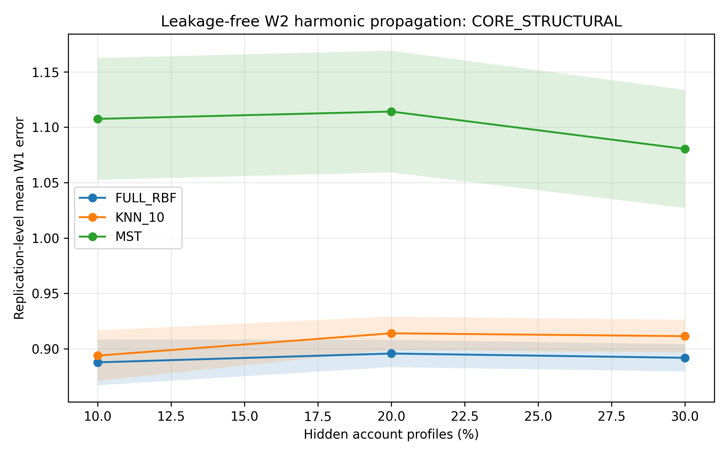
Full RBF yields the lowest mean reconstruction error at all three missingness rates, followed by KNN-10, whereas MST produces appreciably larger errors. At 20% missingness, the mean error is 0.942 for Full RBF (95% confidence interval 0.929–0.954), 0.960 for KNN-10 (0.945–0.975) and 1.190 for MST (1.133–1.247). The corresponding mean errors are 0.896, 0.914 and 1.114.
| Graph | Missing | Mean | 95\ Mean | 95\ Full RBF | 10\ Full RBF | 20\ Full RBF | 30\ KNN-10 | 10\ KNN-10 | 20\ KNN-10 | 30\ MST | 10\ MST | 20\ MST | 30\ |
|---|
Paired comparisons at 20% missingness show that the difference between Full RBF and KNN-10 is modest in magnitude but consistent across the realised masks. The Full RBF minus KNN-10 difference in mean is (95% confidence interval to ; Holm-adjusted ). The corresponding differences are for Full RBF versus MST ( to ) and for KNN-10 versus MST ( to ); both adjusted . Thus, the dense graph performs best in the primary regime, KNN-10 remains close, and restricting connectivity to a spanning tree produces a material loss of accuracy.
Mean error is not monotone in the proportion of hidden profiles. In particular, MST error at 30% missingness is lower than at 10% and 20%. The masks at different missingness rates were generated separately and were not nested. Consequently, cross-rate differences reflect both the amount of missingness and the composition of the hidden sets. No formal paired inference is attached to the apparent non-monotonicity across missingness rates.
Figure e̊f{fig:core_missingness} presents the complementary results. Full RBF and KNN-10 remain close throughout the three conditions, whereas the MST curve is consistently higher. The separation between graph topologies is larger than the variation in their mean errors across missingness rates.
Comparison with benchmark estimators
Table e̊f{tab:baseline_w2} compares the four estimators at the central 20% missingness condition. The Global Probability benchmark has the same mean error across graphs and feature regimes because it does not use graph or covariate information. Its mean error is 1.346.
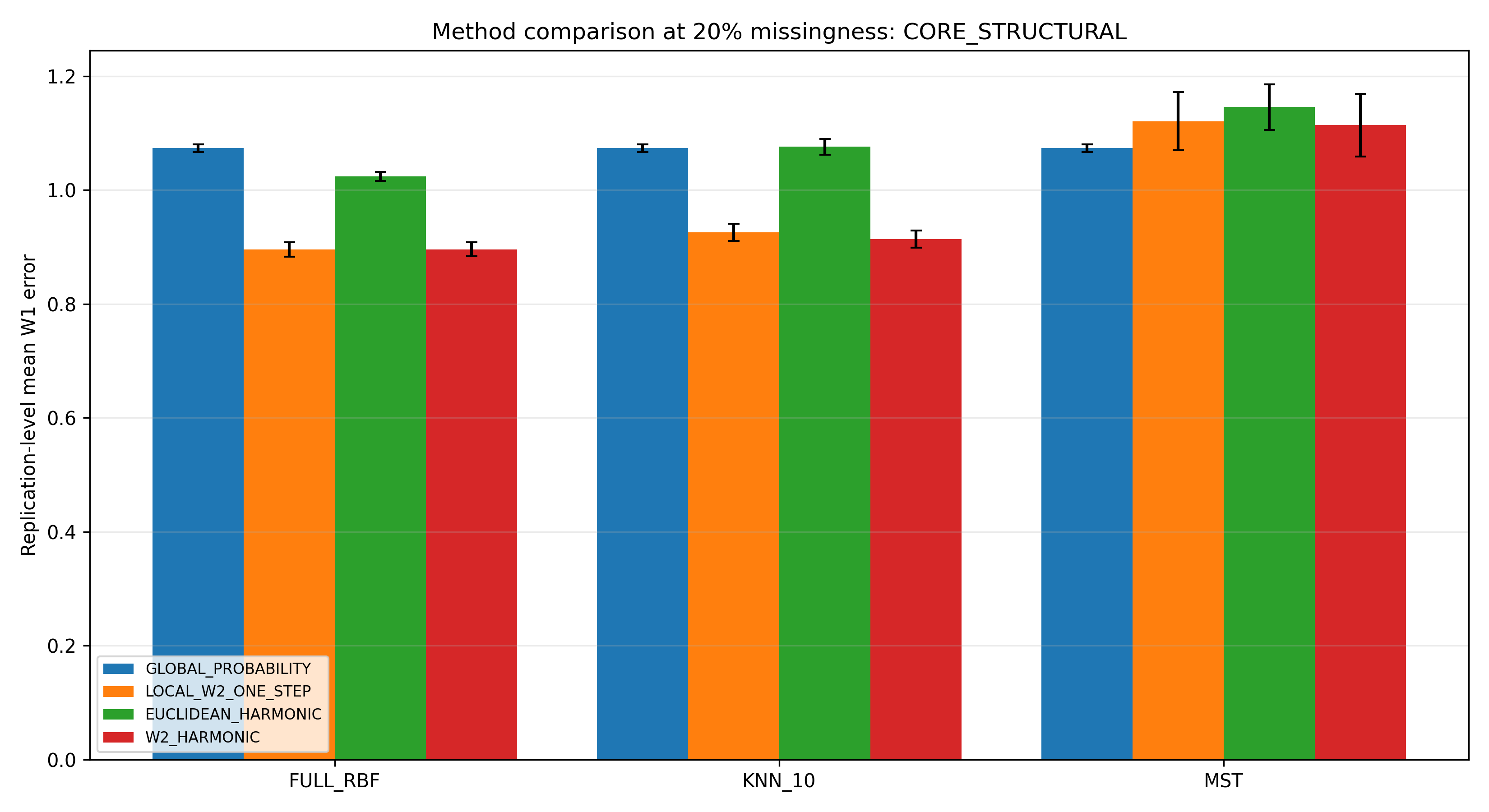
Under the \textsc{Core Structural} regime, -harmonic propagation reduces mean error relative to Global Probability by 30.1% on Full RBF, 28.7% on KNN-10 and 11.6% on MST. Relative to Euclidean Harmonic propagation, the corresponding reductions are 27.3%, 28.3% and 7.2%. The contribution of Wasserstein geometry is therefore substantial on Full RBF and KNN-10 and smaller, although still detectable, on the minimally connected tree.
| Feature regime | Graph | Global | Euclidean harmonic | Local | harmonic | Gain vs.\ global | Gain vs.\ Euclidean | |||||||||||||||||||||||||||||
|---|---|---|---|---|---|---|---|---|---|---|---|---|---|---|---|---|---|---|---|---|---|---|---|---|---|---|---|---|---|---|---|---|---|---|---|---|
| \multirow{3}{*}{Core Structural} | Full RBF | 1.346 | 1.296 | 0.941 | 0.942 | 30.1\ | KNN-10 | 1.346 | 1.340 | 0.974 | 0.960 | 28.7\ | MST | 1.346 | 1.283 | 1.196 | 1.190 | 11.6\ \multirow{3}{*}{Extended Amount Sensitivity} | Full RBF | 1.346 | 0.367 | 0.223 | 0.229 | 83.0\ | KNN-10 | 1.346 | 0.320 | 0.208 | 0.212 | 84.3\ | MST | 1.346 | 0.221 | 0.235 | 0.186 | 86.2\ |
Paired tests support the differences between the two harmonic representations. Relative to Euclidean Harmonic, the mean reduction achieved by Harmonic is 0.354 on Full RBF (95% confidence interval 0.346–0.362), 0.380 on KNN-10 (0.364–0.395) and 0.093 on MST (0.046–0.140). All three comparisons have Holm-adjusted . Respecting the ordinal transport geometry therefore contributes on all three graph topologies, although the relative gain is smaller on MST.
The contrast with Local One-Step is smaller. On Full RBF, the local estimator has a mean error lower by less than 0.0001, and the paired difference is not distinguishable across masks (95% confidence interval to ; adjusted ). On KNN-10, Harmonic reduces mean error by 0.0135 (0.0095–0.0175; adjusted ). On MST, the reduction is 0.0058 (0.0016–0.0100; adjusted ). Accordingly, most of the gain over the global benchmark is obtained by combining account-specific graph neighbourhoods with Wasserstein geometry. Multi-hop propagation provides an additional, but comparatively small, improvement on KNN-10 and MST, while it does not improve on the one-step estimator in the fully connected graph.
Figure e̊f{fig:core_method_comparison} reports the corresponding comparison. It is included as a complementary linear-cost view of the same 20% missingness experiment; the formal paired tests reported above use , the primary metric.
Amount-summary sensitivity analysis
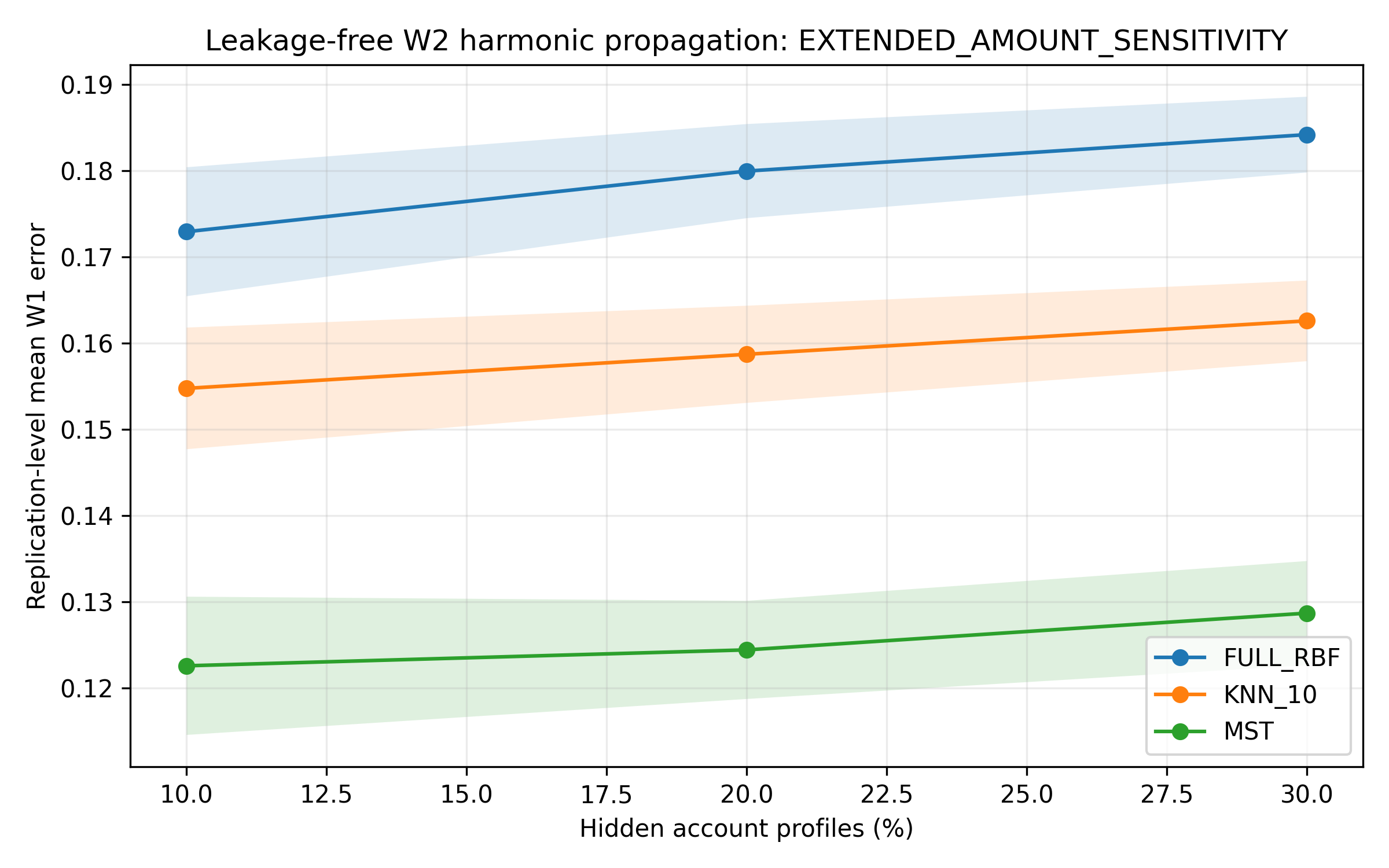
Adding total, mean, median and standard deviation of outgoing amounts to the graph features produces substantially lower reconstruction errors (Table e̊f{tab:extended_results}). At 20% missingness, mean is 0.229 on Full RBF, 0.212 on KNN-10 and 0.186 on MST. Relative to the corresponding \textsc{Core Structural} graphs, these values represent reductions of 75.7%, 77.9% and 84.4%, respectively.
These reductions show that coarse summaries of the underlying amounts contain considerable information about the location and dispersion of the target profile. They should not be interpreted as performance obtainable when all amount-derived information is unavailable. The extended regime is therefore a sensitivity analysis for covariate availability rather than a replacement for the primary structural-only analysis.
| Graph | Missing | Mean | 95\ Mean | 95\ Full RBF | 10\ Full RBF | 20\ Full RBF | 30\ KNN-10 | 10\ KNN-10 | 20\ KNN-10 | 30\ MST | 10\ MST | 20\ MST | 30\ |
|---|
The topology ranking reverses relative to the primary regime. At 20% missingness, Full RBF minus KNN-10 is 0.0173 (95% confidence interval 0.0159–0.0188), Full RBF minus MST is 0.0434 (0.0370–0.0497), and KNN-10 minus MST is 0.0260 (0.0203–0.0318). All three Holm-adjusted -values are below 0.001. MST therefore performs best when graph geometry is constructed using strongly target-aligned amount summaries. This reversal shows that the relative performance of graph topologies depends on the information encoded in the feature space; it is not an intrinsic ordering of Full RBF, KNN-10 and MST.
Within the extended regime, Harmonic also outperforms Euclidean Harmonic on all three graphs. The mean reductions are 0.138 on Full RBF (95% confidence interval 0.135–0.140), 0.108 on KNN-10 (0.105–0.111) and 0.035 on MST (0.033–0.038), with Holm-adjusted in every case.
The comparison with Local One-Step is topology-dependent. On Full RBF, the local estimator is lower than harmonic propagation by 0.0063 (95% confidence interval 0.0058–0.0069), and on KNN-10 it is lower by 0.0041 (0.0030–0.0052). On MST, by contrast, Harmonic reduces error relative to the local estimator by 0.0497 (0.0398–0.0595). All three Holm-adjusted -values are below 0.001. Under the extended feature regime, multi-hop propagation is therefore beneficial on the minimally connected graph but provides no advantage over direct observed neighbours on the denser topologies.
Figure e̊f{fig:extended_missingness} shows that the same topology ordering is present for the complementary metric throughout the three missingness conditions.
Account-level error heterogeneity
Replication-level means conceal substantial heterogeneity among individual account reconstructions. Figure e̊f{fig:w1_boxplot} pools the account-level errors obtained at 20% missingness under the \textsc{Core Structural} regime. Each graph contributes 4,000 account-mask errors: 200 hidden accounts in each of 20 replications.
The pooled median errors are 0.802 for Full RBF, 0.832 for KNN-10 and 1.000 for MST. Their respective 95th percentiles are 1.701, 1.883 and 3.000. The upper tail is therefore materially wider for MST, which reaches the maximum possible displacement of 3 on the ordinal support. The maximum observed errors for Full RBF and KNN-10 are 2.000 and 2.322, respectively.
These pooled errors are used only for descriptive purposes. The same account may be hidden in more than one replication, and errors from accounts within a replication share the same observed boundary conditions. They are therefore not treated as independent observations for confidence intervals or hypothesis tests.
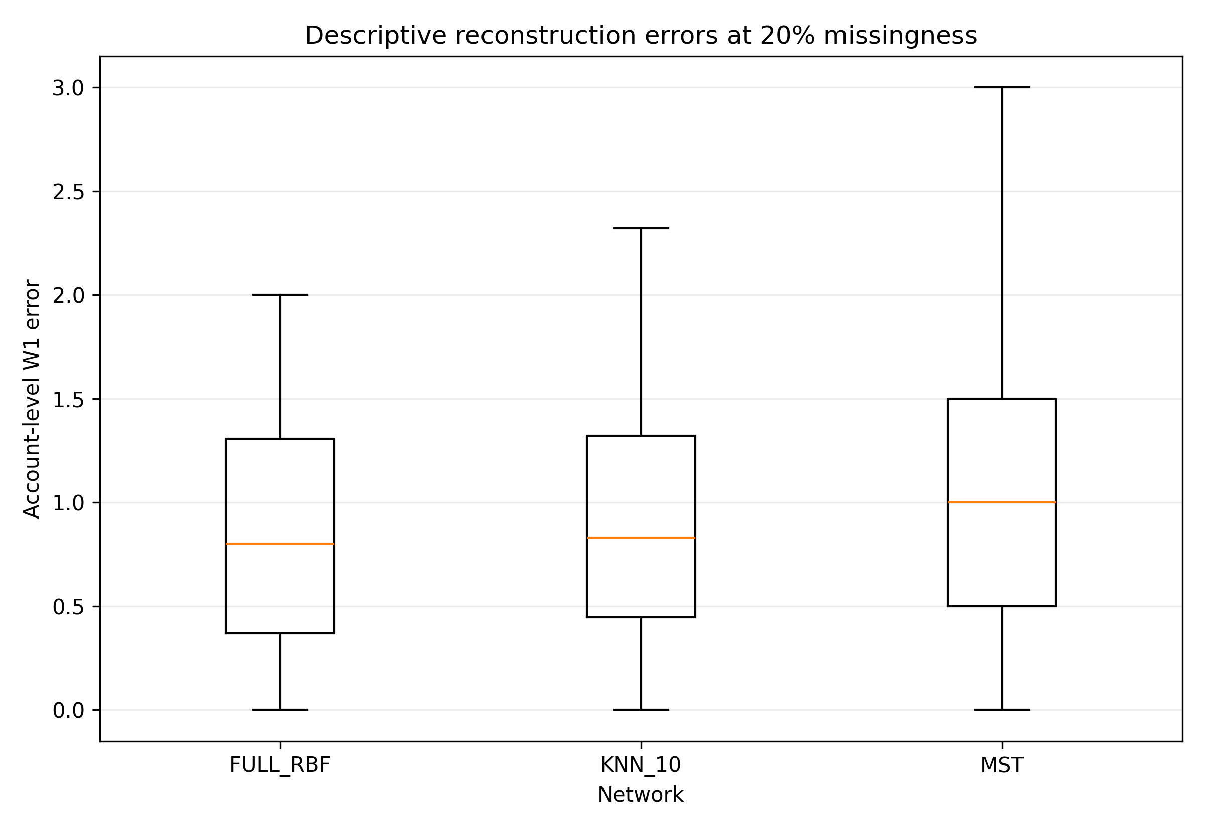
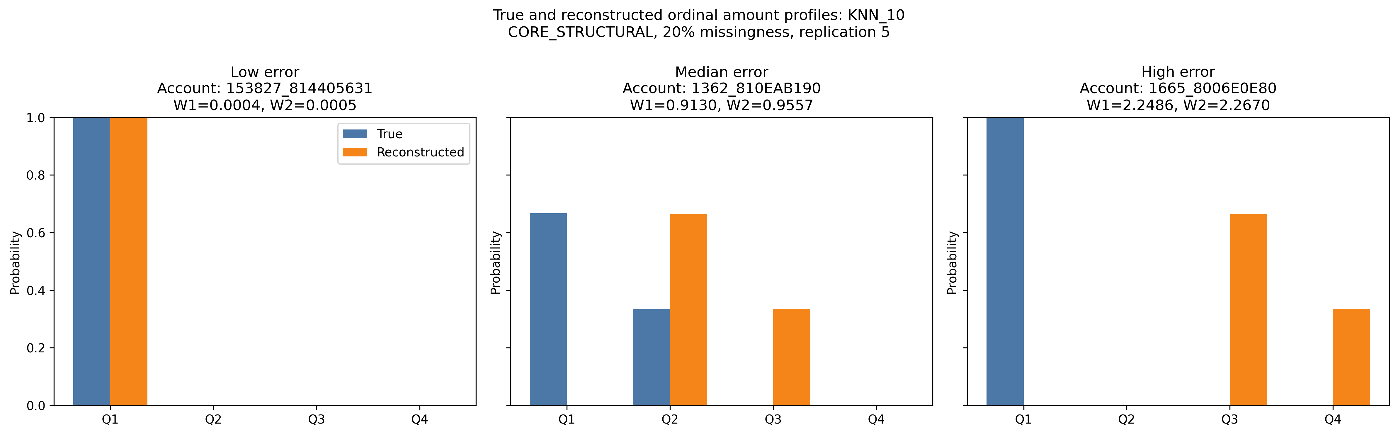
Figure e̊f{fig:knn_cases} examines three KNN-10 reconstructions from replication 5. This replication was selected because its replication-level mean error is closest to the median of the 20 KNN-10 replication means. Within that replication, the displayed accounts correspond to the lowest, median and highest account-level ranks.
The low-error account is a pure-Q1 profile and is recovered almost exactly ( ). The median-error account places two thirds of its mass in Q1 and one third in Q2, whereas the reconstruction places approximately 66.4% in Q2 and 33.6% in Q3 ( ). The high-error account is a pure-Q1 profile, while the reconstruction places approximately 66.4% in Q3 and 33.6% in Q4 ( ). These examples illustrate how similar replication-level averages can coexist with qualitatively different account-level errors.
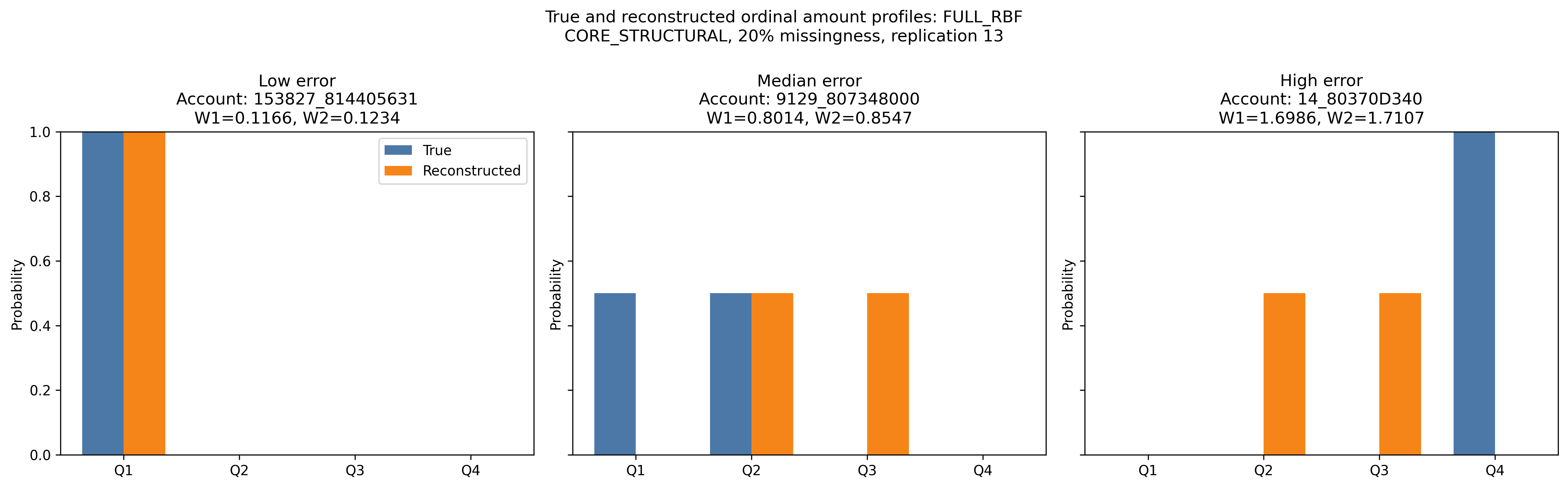
The class probabilities in Figure e̊f{fig:knn_cases} are projections of the continuous predicted quantile functions and are used for visualisation only. All case rankings and numerical errors are calculated in the 128-dimensional quantile representation. Corresponding examples for Full RBF and MST are reported in Figures e̊f{fig:full_cases_appendix} and e̊f{fig:mst_cases_appendix}.
\FloatBarrier \FloatBarrier
Discussion
The results support four main conclusions concerning distributional geometry, propagation depth, feature availability and graph topology. These conclusions are conditional on the fixed synthetic dataset, the selected accounts and the missingness design; they should be read as evidence about the reconstruction experiment rather than as population-level claims about banking behaviour.
First, respecting the geometry of the response materially improves harmonic reconstruction. Under the primary \textsc{Core Structural} regime, the -harmonic estimator reduces mean error relative to Euclidean harmonic smoothing on every graph. At 20% missingness, the reductions are 0.354 on Full RBF, 0.380 on KNN-10 and 0.093 on MST, and all three paired comparisons remain significant after Holm correction. The result is not a generic benefit of increasing response dimensionality: both harmonic methods use the same graph and observed accounts, but only the Wasserstein estimator represents the ordering and displacement between Q1–Q4. A probability vector is therefore not interchangeable with an unconstrained four-dimensional response. In this setting, quantile-space propagation preserves information about how far probability mass must move, which is the central motivation for Wasserstein graph smoothing [9].
Second, Wasserstein geometry and multi-step propagation make distinct contributions. Most of the gain over the global benchmark is already obtained by the Local One-Step estimator, which combines observed neighbour profiles without solving the full harmonic system. Under the core regime, the local and harmonic estimators are effectively tied on Full RBF, where every hidden account is directly connected to all observed accounts. Harmonic propagation provides a small but consistent improvement on KNN-10 and MST, where paths through hidden nodes can supplement direct observed neighbours. Under the extended regime, the local estimator is slightly more accurate on Full RBF and KNN-10, whereas harmonic propagation improves mean error by 0.0497 on MST. This pattern is consistent with the role of harmonic extension as a mechanism for transmitting boundary information through sparse paths [2, 3]; it does not support the stronger claim that deeper propagation is uniformly preferable. A local Wasserstein benchmark is consequently necessary to distinguish gains from distributional averaging from gains attributable specifically to multi-hop diffusion.
Third, the information used to construct the graph has a larger descriptive association with accuracy than the differences observed across the three masking rates. Adding total, mean, median and standard deviation of transaction amounts reduces the -harmonic error by 75.7–84.4% relative to the corresponding structural-only graphs at 20% missingness. These summaries are not the four target probabilities and therefore do not violate the formal feature exclusion imposed by the experiment. They are, however, calculated from the same underlying amounts and strongly constrain the location and dispersion of the missing profile. The extended regime must therefore be interpreted as a different information condition, not as an unqualified improvement over the primary specification. Its relevance depends on the deployment setting: it is appropriate when an account histogram is unavailable but coarser amount summaries remain observable, and inappropriate when all amount-derived information is missing.
Fourth, topology cannot be assessed independently of the feature space from which affinities are constructed. Full RBF performs best in the primary structural-only regime, KNN-10 remains close, and MST is materially less accurate. When amount summaries are included, the ordering reverses and MST has the lowest mean error. This reversal does not establish that dense graphs are intrinsically robust or that spanning trees are intrinsically preferable with informative covariates. It shows instead that the same edge-retention rule induces a different smoothing operator when feature distances and affinity weights change. In particular, the two Full RBF graphs retain the same 499,500 edges but have markedly different mean weighted degrees. Edge count alone is therefore insufficient to characterise effective connectivity or smoothing strength. The finding is consistent with the broader observation that graph construction is part of the model rather than a neutral preprocessing choice [4, 16].
The core KNN-10 graph provides an additional qualification. It contains five connected components, yet each component retained at least one observed profile in every realised mask and no fallback prediction was required. Its performance therefore reflects component-wise harmonic reconstruction under the reported random masks. More structured missingness could remove all observed anchors from a component, in which case reconstruction would depend on the specified global fallback rather than on within-component propagation. Connectivity diagnostics should consequently accompany accuracy measures when the method is applied to sparse graphs.
Mean errors also conceal substantial account-level heterogeneity. At 20% missingness under the core regime, the pooled median errors are 0.802, 0.832 and 1.000 for Full RBF, KNN-10 and MST, whereas their 95th percentiles are 1.701, 1.883 and 3.000. The representative KNN-10 cases further show that concentrated profiles can be reconstructed almost exactly or displaced by more than two ordinal classes. Thus, similar replication-level means can coexist with materially different account-level outcomes. For applications in which individual reconstructions would inform downstream decisions, reporting only an average error would be inadequate; tail behaviour, account-level uncertainty and rules for abstaining from poorly supported predictions would also be required.
Errors are comparatively stable across the examined 10%, 20% and 30% missingness conditions, but they are not monotone. The masks were generated separately at each rate rather than nested, so cross-rate differences combine the amount of missingness with changes in the composition and difficulty of the hidden accounts. The experiment therefore supports only the limited claim that average performance remains of a similar order across these three random-mask conditions. It does not establish insensitivity to progressively increasing missingness, nor does it describe performance under clustered, component-wise or informative missingness.
Finally, the analysis concerns reconstruction rather than AML detection. The method does not use illicit-activity labels, and Q1–Q4 indicate positions in the pooled amount distribution rather than levels of suspicion or regulatory risk. The behavioural graph is likewise a similarity graph constructed from account-level covariates, not the directed network of observed transfers. Accurate profile reconstruction should not be interpreted as evidence of fraud detection, causal peer influence or privacy protection. Aggregation does not itself provide a formal privacy guarantee, and reconstructed profiles may remain sensitive account-level information.
Within these boundaries, the study extends Wasserstein propagation to a financial account-level setting and provides a controlled assessment of when its gains arise. The strongest empirical support concerns the use of distribution-aware geometry relative to Euclidean harmonic smoothing. The incremental value of multi-step propagation is more conditional, and the much larger gains obtained from amount summaries demonstrate why feature availability and leakage-aware benchmark design must be stated explicitly.
Limitations and Future Work
The study has several limitations that delimit the interpretation of the reported results and motivate extensions of the present framework.
First, the empirical analysis uses a single synthetic benchmark. The IBM HI-Small data provide a large, fully labelled and reproducible environment, but the dependence among activity intensity, counterparties, payment formats and transaction amounts is generated rather than observed in a regulated financial institution. The 18-day observation window also provides no evidence about longer-run temporal stability. External validation should therefore examine appropriately governed real data from multiple periods or institutions and report whether graph construction, topology rankings and reconstruction accuracy transport across settings. Such validation would require institution-specific privacy, access and governance controls and should not assume that the relationships found in the synthetic benchmark remain unchanged.
Second, transaction amounts are analysed in the numerical scale supplied by the source data. The transaction-level records contain currency identifiers, but the preprocessing used in this study does not convert amounts to a common currency before constructing the global quartiles. The resulting Q1–Q4 classes describe relative positions in the pooled numerical field rather than purchasing-power-comparable monetary values. Future preprocessing should either convert amounts using transaction-date exchange rates, construct currency-specific profiles, or normalise amounts within currency before aggregation. The choice among these alternatives changes the interpretation of the target and should be specified before graph construction and masking.
The four-class representation introduces a related approximation. Unit ground distance on treats a movement across one class boundary as one ordinal step, even though the monetary gaps associated with the global quartiles are unequal. This is intentional in the present study because the classes encode order rather than cardinal monetary distance, but the resulting and values should be interpreted on the ordinal-class scale. Future work could compare alternative numbers of bins, data-driven support locations, log-amount ground metrics and continuous amount distributions. These alternatives would define different reconstruction targets and should be evaluated as sensitivity analyses rather than treated as interchangeable parameterisations.
Third, the observed account histogram is treated as the reconstruction target without modelling its sampling uncertainty. Even with the eligibility rule , an empirical profile based on a finite number of transactions is only an estimate of the account's latent behavioural distribution. This issue is particularly relevant for low-activity accounts and for the many selected profiles concentrated in a single class. The reported errors therefore measure recovery of the realised empirical profile, not recovery of an unobserved long-run account distribution. Hierarchical multinomial models, profile shrinkage or bootstrap procedures could separate uncertainty in the underlying account distribution from error introduced by graph-based reconstruction.
Fourth, the masking mechanism is imposed uniformly at random within the fixed sample. It is consequently analogous to account-level missing completely at random and does not represent the selective missingness likely to occur in practice. Profile availability may depend on institution, product, activity, data-provider coverage, graph component or the unobserved profile itself. Future experiments should include feature-dependent masks, activity-blocked masks, entire unobserved components and controlled missing-not-at-random mechanisms. Nested masks would also permit a direct assessment of deterioration as missingness increases. The present 20 replications quantify variation over the chosen random masks conditional on one fixed sample and graph; they do not capture variation across datasets, institutions or time periods.
Fifth, the experiment is transductive. All 1,000 accounts and their non-target covariates are available when feature transformations, local scales and graph edges are constructed. The evaluation therefore does not test prediction for a newly arriving account outside the fitted graph. An operational system would require either rebuilding the graph, defining an out-of-sample rule for connecting new accounts, or learning an inductive mapping from covariates to distributional profiles. Fréchet regression for random objects provides one general route for covariate-based distributional prediction [1], while graph-aware inductive extensions would need to retain the leakage controls used in the present design.
Sixth, the analysis is conditional on an activity-stratified sample of 1,000 accounts selected from senders with at least 20 outgoing transactions. It does not establish performance for low-activity accounts or for the full eligible population. The sample also makes dense Full RBF construction computationally manageable; applying the same procedure to 100,229 eligible accounts would require more than five billion pairwise affinities before reconstruction. Scalable extensions could use approximate nearest-neighbour search, sparse or landmark graphs, Nyström approximations and iterative Laplacian solvers. Evaluation should then report both computational error and reconstruction error, rather than assuming that the approximate graph reproduces the present topology.
Seventh, the estimator relies on a graph-smoothness assumption: accounts close in the selected feature space are expected to have similar amount profiles. Only three structural covariates are used in the primary graph, and their similarity need not imply similarity of the target distribution. Conversely, the extended amount summaries are strongly target-aligned and are useful only when they remain observable under the intended missing-data scenario. The graphs are also static, undirected similarity networks; they do not represent the direction, multiplicity or timing of actual transfers. Future work could compare similarity and transaction-flow graphs, construct multiplex networks, and model profile evolution over rolling time windows. Any temporal extension should construct features and edges using information available before the prediction time to avoid look-ahead leakage.
Eighth, the graph and numerical hyperparameters are fixed rather than selected through a nested validation design. These choices include the number of nearest neighbours, the local-scale order, the affinity kernel, the quantile-grid resolution and the numerical ridge. Although fixed settings support a controlled comparison, they do not establish optimality or robustness to alternative specifications. Future studies should prespecify a hyperparameter search and perform selection using only information available within each training mask. Repeated account samples, rather than repeated masks alone, would additionally reveal sensitivity to the realised node set.
Finally, the method produces point reconstructions but no account-specific measure of predictive uncertainty. Confidence intervals across replication means quantify Monte Carlo variation in average performance and are not prediction intervals for individual profiles. Wasserstein inference and simultaneous confidence bands developed for Fréchet regression provide relevant methodological precedents [19], but they do not directly account for graph dependence, empirical-histogram uncertainty or uncertainty in graph construction. Extending inference to this setting is therefore a substantive problem rather than a direct application of existing bands. Future work should evaluate coverage, tail risk and abstention rules so that poorly supported account-level reconstructions can be identified rather than reported with the same apparent certainty as well-supported predictions.
Conclusion
This paper has examined the reconstruction of partially observed account-level transaction-amount distributions on behavioural similarity graphs. The proposed approach represents each empirical distribution through its one-dimensional quantile function and formulates reconstruction as a graph-harmonic boundary-value problem under squared geometry. The experimental design separates the target profile from all graph-construction operations and evaluates global, local, Euclidean and Wasserstein estimators under identical account masks.
The primary structural-only analysis shows that distributional geometry matters. At 20% missingness, -harmonic propagation reduces mean error relative to both global probability averaging and Euclidean harmonic smoothing on all three graph topologies. The size of the improvement varies with connectivity and is smallest on the minimum spanning tree. At the same time, the comparison with the one-step Wasserstein estimator qualifies the role of propagation depth: the two estimators are effectively tied on Full RBF, and the additional benefit of multi-step diffusion is modest on the core KNN-10 and MST graphs. The evidence therefore supports Wasserstein geometry more strongly than it supports a universal advantage of harmonic propagation over direct distributional averaging among observed neighbours.
The extended analysis further shows that graph performance cannot be separated from feature availability. When total, mean, median and standard deviation of transaction amounts remain observable, reconstruction errors fall sharply and MST becomes the most accurate topology. These results describe a richer, target-aligned information regime and should not replace the structural-only findings. Instead, the reversal demonstrates that the graph, the estimator and the assumed missing-data scenario form a single modelling specification.
The main contribution is consequently both methodological and evaluative. Quantile-space harmonic extension provides a tractable way to reconstruct ordered probability distributions, while the leakage-aware benchmark reveals which improvements arise from distributional geometry, graph propagation and side information. Within the limits of the synthetic, transductive experiment, the results support Wasserstein-based reconstruction as a useful approach to missing distributional summaries. They do not establish AML detection, account-level risk classification, causal network effects or performance in an operational banking environment. Establishing those broader claims requires real-data validation, alternative missingness mechanisms, scalable graph construction and account-level uncertainty quantification.
Data and Code Availability
The study uses the public synthetic IBM Transactions for Anti-Money Laundering benchmark introduced by [11]. The raw transaction data are not redistributed with this manuscript and must be obtained from the original provider under the applicable data licence.
The reproducibility package accompanying the manuscript contains the account-level analytical input used by the final experiment, the executable analysis notebook and Python scripts, the fixed configuration, the selected account sample and its checksum, graph diagnostics, replication- and account-level errors, paired statistical tests, reproducibility checks and the reported figures. These materials reproduce the sampling, graph construction, masking, estimation, evaluation and visualisation stages from the supplied account-level input. The current package does not yet include the upstream script that converts the raw transaction file into that account-level input; this preprocessing script and a permanent repository identifier should be added before public release.
Acknowledgements
To be completed before submission with funding, institutional and collaborator acknowledgements, where applicable.
Reproducibility Checklist
Table e̊f{tab:reproducibility_settings} records the analytical settings used for the reported results. These settings are fixed in the final configuration and are shared across all paired comparisons unless stated otherwise.
| Setting | Value | |
|---|---|---|
| Account-level input | \path{account_amount_distributions.csv} | |
| Pseudorandom seed | 123 | |
| Minimum outgoing transactions for eligibility | 20 | |
| Selected accounts | 1,000 | |
| Activity strata and quota | 10 strata; 100 accounts per stratum | |
| Feature regimes | Core Structural; Extended Amount Sensitivity | |
| Graph topologies | Full RBF; KNN-10; MST | |
| Reconstruction methods | Global Probability; Local One-Step; Euclidean Harmonic; Harmonic | |
| Feature transformation | for non-negative covariates | |
| Missing-feature rule | Feature-wise median imputation | |
| Feature scaling | Zero mean and unit variance | |
| Quantile grid | 128 midpoint probabilities | |
| Missingness rates | 0.10, 0.20 and 0.30 | |
| Hidden accounts per replication | 100, 200 and 300, respectively | |
| Replications per missingness rate | 20 | |
| KNN neighbourhood size | 10 | |
| Local RBF scale | Tenth-nearest-neighbour distance | |
| Numerical harmonic ridge | ||
| Unanchored-component fallback | Mean observed representation; never activated | |
| Primary response metric | Discretised error | |
| Secondary response metric | Discretised error | |
| Monte Carlo unit | Mean error within each replication | |
| Interval summary | Two-sided 95\ Paired tests | Two-sided Wilcoxon signed-rank tests |
| Multiplicity adjustment | Holm correction within each prespecified comparison family | |
| Primary inferential condition | 20\ |
All numerical errors are evaluated directly on the 128-dimensional predicted quantile vectors after range and monotonicity correction. Projection of a continuous predicted quantile function onto Q1–Q4 probabilities is used only for visualisation and does not enter the numerical evaluation, confidence intervals or paired tests.
The final run passed all 13 automated reproducibility checks. These checks verify the selected-account count and uniqueness, unit profile sums, the complete grid of 72 experimental configurations, the expected hidden-account counts, finite replication metrics, absence of unanchored components, complete paired-test grids, valid adjusted -values and the presence of every required figure. The exact results are recorded in \path{reproducibility_checks.csv}.
The selected sample and its ordering are identified by the SHA-256 digest e̱gin{center} \nolinkurl{767ffcd0ccb1bf9f1e52513bb641dd2014250a9af94adc61077e3b20e00c9caa}. \end{center} The executable configuration is stored in \path{analysis_config.json}, and \path{run_manifest.json} records the execution environment. The reported run used Python 3.13.15, NumPy 2.1.3, pandas 2.2.3, SciPy 1.16.3, scikit-learn 1.6.1, NetworkX 3.6.1 and Matplotlib 3.10.0.
\FloatBarrier
Additional Representative Reconstructions
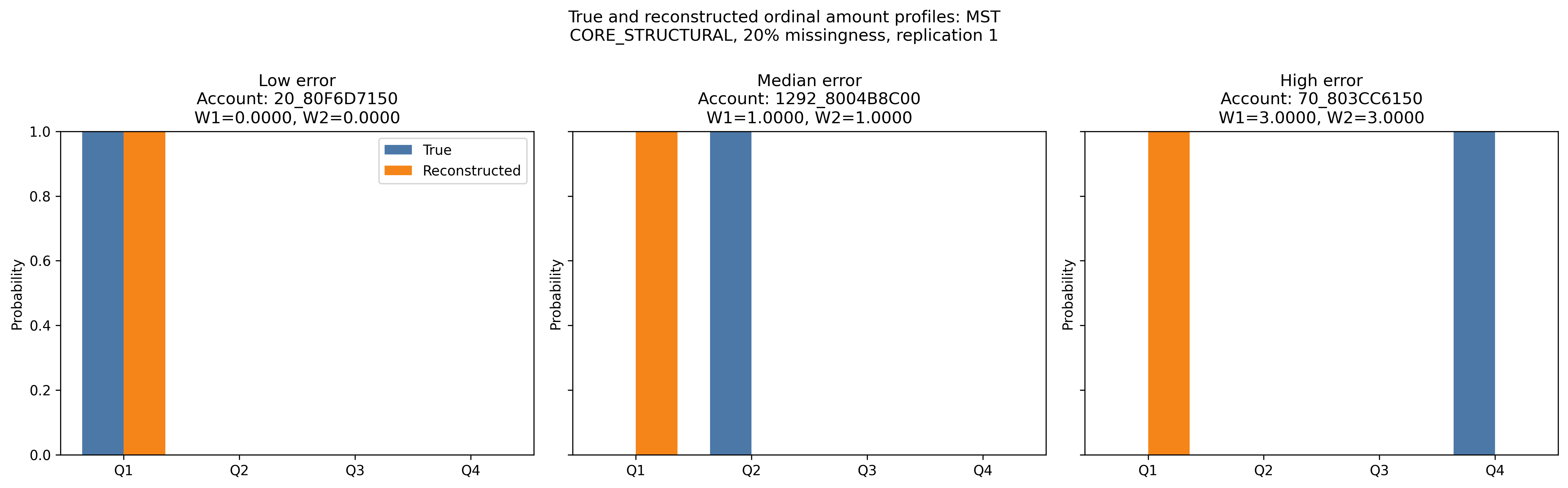
Section e̊f{subsec:error_heterogeneity} reports representative KNN-10 cases. For completeness, Figures e̊f{fig:full_cases_appendix} and e̊f{fig:mst_cases_appendix} present the corresponding Full RBF and MST reconstructions. For each graph, the displayed replication is the one whose mean error is closest to the median of the 20 replication-level means at 20% missingness under the \textsc{Core Structural} regime. Within that replication, the three accounts correspond to the lowest, median and highest account-level ranks. The displayed class probabilities are projections used for visualisation; case selection and error calculation use the original 128-dimensional quantile vectors.
\FloatBarrier
Interpretation of the Ordinal Ground Metric
The four amount classes are embedded in the ordered support
This ground metric assigns unit cost to movement between adjacent classes and a cost of three to movement between Q1 and Q4. Consequently, both and range from zero to three for distributions supported entirely on the four class locations. Their numerical values are expressed in ordinal-class units, not in currency units.
The unit-spacing convention encodes only the ordering of Q1–Q4. It does not assert that the underlying monetary distance between Q1 and Q2 equals that between Q3 and Q4. This distinction is important because the empirical quartile boundaries are unequally spaced on the supplied amount scale and the source transactions include multiple currencies without a common conversion in the analytical file. Using ordinal support prevents large raw numerical amounts from mechanically dominating the transport cost, but it also removes information about the cardinal size of monetary displacements.
Alternative ground geometries could locate each class at a representative log-amount, use currency-adjusted class centroids, construct separate within-currency supports or retain continuous converted amounts. Such choices would change the estimand as well as the scale of the errors. They may also alter neighbourhood performance and the relative ranking of graph topologies, particularly under the amount-summary feature regime. Comparisons across ground metrics should therefore report both the support definition and its units rather than interpreting the resulting Wasserstein errors as directly interchangeable.
Bibliography
References
- . Fréchet Regression for Random Objects with Euclidean Predictors. The Annals of Statistics, 47(2), pp. 691–719, 2019.DOI ↗
- . Semi-Supervised Learning Using Gaussian Fields and Harmonic Functions. Proceedings of the 20th International Conference on Machine Learning, pp. 912–919, 2003.Source ↗
- . Learning with Local and Global Consistency. Advances in Neural Information Processing Systems, 16, pp. 321–328, 2004.Source ↗
- . Manifold Regularization: A Geometric Framework for Learning from Labeled and Unlabeled Examples. Journal of Machine Learning Research, 7(85), pp. 2399–2434, 2006.Source ↗
- . Optimal Transport: Old and New. Springer, 338, 2009.DOI ↗
- . Computational Optimal Transport: With Applications to Data Science. Foundations and Trends in Machine Learning, 11(5–6), pp. 355–607, 2019.DOI ↗
- . Statistical Aspects of Wasserstein Distances. Annual Review of Statistics and Its Application, 6, pp. 405–431, 2019.DOI ↗
- . Barycenters in the Wasserstein Space. SIAM Journal on Mathematical Analysis, 43(2), pp. 904–924, 2011.DOI ↗
- . Wasserstein Propagation for Semi-Supervised Learning. Proceedings of the 31st International Conference on Machine Learning, 32(1), pp. 306–314, 2014.Source ↗
- . A Network-Based Distributional Inference Approach to Model Country-Level Cyber Risk. Journal of the Royal Statistical Society Series A: Statistics in Society, pp. qnag049, 2026.DOI ↗
- . Realistic Synthetic Financial Transactions for Anti-Money Laundering Models. Advances in Neural Information Processing Systems, 36, 2023.DOI ↗
- . Collective Fraud Detection Capturing Inter-Transaction Dependency. Proceedings of the KDD 2017: Workshop on Anomaly Detection in Finance, 71, pp. 66–75, 2018.Source ↗
- . Anti-Money Laundering in Bitcoin: Experimenting with Graph Convolutional Networks for Financial Forensics. arXiv preprint arXiv:1908.02591, 2019.Source ↗
- . Provably Powerful Graph Neural Networks for Directed Multigraphs. Proceedings of the AAAI Conference on Artificial Intelligence, 38(10), pp. 11838–11846, 2024.DOI ↗
- . Self-Tuning Spectral Clustering. Advances in Neural Information Processing Systems, 17, pp. 1601–1608, 2004.Source ↗
- . A Tutorial on Spectral Clustering. Statistics and Computing, 17, pp. 395–416, 2007.DOI ↗
- . Individual Comparisons by Ranking Methods. Biometrics Bulletin, 1(6), pp. 80–83, 1945.DOI ↗
- . A Simple Sequentially Rejective Multiple Test Procedure. Scandinavian Journal of Statistics, 6(2), pp. 65–70, 1979.
- . Wasserstein $F$-Tests and Confidence Bands for the Fréchet Regression of Density Response Curves. The Annals of Statistics, 49(1), pp. 590–611, 2021.DOI ↗